Robótica

Clase 07

Semana 8 - 05/05/2025

Posicionamiento 2D

Posicionamiento 2D

Posicionamiento 2D

Posicionamiento 2D

Posicionamiento 2D

Posicionamiento 2D

Posicionamiento 2D

Posicionamiento 2D

Posicionamiento 2D

Posicionamiento 2D

Posicionamiento 2D

Marcos de referencia: cómo convertirmos coordenadas entre ellos?

Notación

• Punto: \(\require{color} \textcolor{PineGreen}{d}_{2D} = \begin{pmatrix} \textcolor{Orange}{a} \\ \textcolor{RedViolet}{b} \end{pmatrix} \;\)

• Vector: \[\require{color} {}^{\textcolor{Blue}{A}}{\boldsymbol{\textcolor{LimeGreen}{p}}_\textcolor{PineGreen}{d}} = \textcolor{Orange}{a} \boldsymbol{\vec{i}} + \textcolor{RedViolet}{b} \boldsymbol{\vec{j}}\]

Transformaciones lineales

Funciones de la forma:

\[ f(\boldsymbol{p}) = \boldsymbol{T} \, \boldsymbol{p} \]

donde \(\boldsymbol{T}\) será una matrix de \(n \times n\), y \(n\) la dimensión de \(\boldsymbol{p}\)

Propiedad

Se pueden encadenar como producto de matrices \[f_3(f_2(f_1(\boldsymbol{p}))) = \boldsymbol{T}_3 \, \boldsymbol{T}_2 \, \boldsymbol{T}_1 \, \boldsymbol{p}\]

Transformaciones lineales

Para el caso 2D

\[ \boldsymbol{T} = \begin{bmatrix} a & b \\ c & d \end{bmatrix} \]

entonces, dado \(\boldsymbol{p} = \begin{bmatrix} x_1 & y_1 \end{bmatrix}^T\)

\[ f(\boldsymbol{p}) = \begin{bmatrix} x_2 \\ y_2 \end{bmatrix} = \begin{bmatrix} a & b \\ c & d \end{bmatrix} \begin{bmatrix} x_1 \\ y_1 \end{bmatrix} = \begin{bmatrix} a x_1 + b y_1 \\ c x_1 + d y_1\end{bmatrix} \]

Rotación 2D

Dado un marco de referencia \(\textcolor{Orange}{\{B\}}\) rotado un ángulo \(\textcolor{Plum}{\theta}\) respecto de un marco de referencia \(\textcolor{Blue}{\{A\}}\). Encontrar la matriz de transformación que convierte las coordenadas del marco \(\textcolor{Orange}{B}\) al \(\textcolor{Blue}{A}\).

Rotación 2D

\[ {}^{\textcolor{Orange}{\boldsymbol{B}}}{\textcolor{ForestGreen}{\boldsymbol{p}}} = \begin{pmatrix} \textcolor{Orange}{p_{{x}_\boldsymbol{B}}} \\ \textcolor{Orange}{p_{{y}_\boldsymbol{B}}} \end{pmatrix} = \begin{pmatrix} \colorbox{white}{$ |\textcolor{ForestGreen}{\boldsymbol{p}}| \cos{\textcolor{Maroon}{\alpha}} $} \\ \colorbox{white}{$ |\textcolor{ForestGreen}{\boldsymbol{p}}| \sin{\textcolor{Maroon}{\alpha}} $} \end{pmatrix} \]

\[ {}^{\textcolor{Blue}{\boldsymbol{A}}}{\textcolor{ForestGreen}{\boldsymbol{p}}} = \begin{pmatrix} \textcolor{Blue}{p_{{x}_\boldsymbol{A}}} \\ \textcolor{Blue}{p_{{y}_\boldsymbol{A}}} \end{pmatrix} = \begin{pmatrix} |\textcolor{ForestGreen}{\boldsymbol{p}}| \cos{(\textcolor{Maroon}{\alpha}+\textcolor{Plum}{\theta})} \\ |\textcolor{ForestGreen}{\boldsymbol{p}}| \sin{(\textcolor{Maroon}{\alpha}+\textcolor{Plum}{\theta})} \end{pmatrix} \]

Sabiendo:

• \(\sin{(A+B)} = \sin{A} \cos{B} + \cos{A} \sin{B}\)
• \(\cos{(A+B)} = \cos{A} \cos{B} - \sin{A} \sin{B}\)

\[ \begin{align} \begin{pmatrix} \textcolor{Blue}{p_{{x}_\boldsymbol{A}}} \\ \textcolor{Blue}{p_{{y}_\boldsymbol{A}}} \end{pmatrix} &= \begin{pmatrix} |\textcolor{ForestGreen}{\boldsymbol{p}}| ( \cos{\textcolor{Maroon}{\alpha}} \cos{\textcolor{Plum}{\theta}} - \sin{\textcolor{Maroon}{\alpha}} \sin{\textcolor{Plum}{\theta}} ) \\ |\textcolor{ForestGreen}{\boldsymbol{p}}| ( \sin{\textcolor{Maroon}{\alpha}} \cos{\textcolor{Plum}{\theta}} + \cos{\textcolor{Maroon}{\alpha}} \sin{\textcolor{Plum}{\theta}} ) \end{pmatrix} \\ &= \begin{pmatrix} \colorbox{white}{$ |\textcolor{ForestGreen}{\boldsymbol{p}}| \cos{\textcolor{Maroon}{\alpha}} $} \cos{\textcolor{Plum}{\theta}} - \colorbox{white}{$ |\textcolor{ForestGreen}{\boldsymbol{p}}| \sin{\textcolor{Maroon}{\alpha}} $} \sin{\textcolor{Plum}{\theta}} \\ \colorbox{white}{$ |\textcolor{ForestGreen}{\boldsymbol{p}}| \sin{\textcolor{Maroon}{\alpha}} $} \cos{\textcolor{Plum}{\theta}} + \colorbox{white}{$ |\textcolor{ForestGreen}{\boldsymbol{p}}| \cos{\textcolor{Maroon}{\alpha}} $} \sin{\textcolor{Plum}{\theta}} \end{pmatrix} \end{align} \]

Rotación 2D

\[ {}^{\textcolor{Orange}{\boldsymbol{B}}}{\textcolor{ForestGreen}{\boldsymbol{p}}} = \begin{pmatrix} \textcolor{Orange}{p_{{x}_\boldsymbol{B}}} \\ \textcolor{Orange}{p_{{y}_\boldsymbol{B}}} \end{pmatrix} = \begin{pmatrix} \colorbox{Gray}{$ |\textcolor{ForestGreen}{\boldsymbol{p}}| \cos{\textcolor{Maroon}{\alpha}} $} \\ \colorbox{white}{$ |\textcolor{ForestGreen}{\boldsymbol{p}}| \sin{\textcolor{Maroon}{\alpha}} $} \end{pmatrix} \]

\[ {}^{\textcolor{Blue}{\boldsymbol{A}}}{\textcolor{ForestGreen}{\boldsymbol{p}}} = \begin{pmatrix} \textcolor{Blue}{p_{{x}_\boldsymbol{A}}} \\ \textcolor{Blue}{p_{{y}_\boldsymbol{A}}} \end{pmatrix} = \begin{pmatrix} |\textcolor{ForestGreen}{\boldsymbol{p}}| \cos{(\textcolor{Maroon}{\alpha}+\textcolor{Plum}{\theta})} \\ |\textcolor{ForestGreen}{\boldsymbol{p}}| \sin{(\textcolor{Maroon}{\alpha}+\textcolor{Plum}{\theta})} \end{pmatrix} \]

Sabiendo:

• \(\sin{(A+B)} = \sin{A} \cos{B} + \cos{A} \sin{B}\)
• \(\cos{(A+B)} = \cos{A} \cos{B} - \sin{A} \sin{B}\)

\[ \begin{align} \begin{pmatrix} \textcolor{Blue}{p_{{x}_\boldsymbol{A}}} \\ \textcolor{Blue}{p_{{y}_\boldsymbol{A}}} \end{pmatrix} &= \begin{pmatrix} |\textcolor{ForestGreen}{\boldsymbol{p}}| ( \cos{\textcolor{Maroon}{\alpha}} \cos{\textcolor{Plum}{\theta}} - \sin{\textcolor{Maroon}{\alpha}} \sin{\textcolor{Plum}{\theta}} ) \\ |\textcolor{ForestGreen}{\boldsymbol{p}}| ( \sin{\textcolor{Maroon}{\alpha}} \cos{\textcolor{Plum}{\theta}} + \cos{\textcolor{Maroon}{\alpha}} \sin{\textcolor{Plum}{\theta}} ) \end{pmatrix} \\ &= \begin{pmatrix} \colorbox{Gray}{$ |\textcolor{ForestGreen}{\boldsymbol{p}}| \cos{\textcolor{Maroon}{\alpha}} $} \cos{\textcolor{Plum}{\theta}} - \colorbox{white}{$ |\textcolor{ForestGreen}{\boldsymbol{p}}| \sin{\textcolor{Maroon}{\alpha}} $} \sin{\textcolor{Plum}{\theta}} \\ \colorbox{white}{$ |\textcolor{ForestGreen}{\boldsymbol{p}}| \sin{\textcolor{Maroon}{\alpha}} $} \cos{\textcolor{Plum}{\theta}} + \colorbox{Gray}{$ |\textcolor{ForestGreen}{\boldsymbol{p}}| \cos{\textcolor{Maroon}{\alpha}} $} \sin{\textcolor{Plum}{\theta}} \end{pmatrix} \end{align} \]

Rotación 2D

\[ {}^{\textcolor{Orange}{\boldsymbol{B}}}{\textcolor{ForestGreen}{\boldsymbol{p}}} = \begin{pmatrix} \textcolor{Orange}{p_{{x}_\boldsymbol{B}}} \\ \textcolor{Orange}{p_{{y}_\boldsymbol{B}}} \end{pmatrix} = \begin{pmatrix} \colorbox{Gray}{$ |\textcolor{ForestGreen}{\boldsymbol{p}}| \cos{\textcolor{Maroon}{\alpha}} $} \\ \colorbox{lightgray}{$ |\textcolor{ForestGreen}{\boldsymbol{p}}| \sin{\textcolor{Maroon}{\alpha}} $} \end{pmatrix} \]

\[ {}^{\textcolor{Blue}{\boldsymbol{A}}}{\textcolor{ForestGreen}{\boldsymbol{p}}} = \begin{pmatrix} \textcolor{Blue}{p_{{x}_\boldsymbol{A}}} \\ \textcolor{Blue}{p_{{y}_\boldsymbol{A}}} \end{pmatrix} = \begin{pmatrix} |\textcolor{ForestGreen}{\boldsymbol{p}}| \cos{(\textcolor{Maroon}{\alpha}+\textcolor{Plum}{\theta})} \\ |\textcolor{ForestGreen}{\boldsymbol{p}}| \sin{(\textcolor{Maroon}{\alpha}+\textcolor{Plum}{\theta})} \end{pmatrix} \]

Sabiendo:

• \(\sin{(A+B)} = \sin{A} \cos{B} + \cos{A} \sin{B}\)
• \(\cos{(A+B)} = \cos{A} \cos{B} - \sin{A} \sin{B}\)

\[ \begin{align} \begin{pmatrix} \textcolor{Blue}{p_{{x}_\boldsymbol{A}}} \\ \textcolor{Blue}{p_{{y}_\boldsymbol{A}}} \end{pmatrix} &= \begin{pmatrix} |\textcolor{ForestGreen}{\boldsymbol{p}}| ( \cos{\textcolor{Maroon}{\alpha}} \cos{\textcolor{Plum}{\theta}} - \sin{\textcolor{Maroon}{\alpha}} \sin{\textcolor{Plum}{\theta}} ) \\ |\textcolor{ForestGreen}{\boldsymbol{p}}| ( \sin{\textcolor{Maroon}{\alpha}} \cos{\textcolor{Plum}{\theta}} + \cos{\textcolor{Maroon}{\alpha}} \sin{\textcolor{Plum}{\theta}} ) \end{pmatrix} \\ &= \begin{pmatrix} \colorbox{Gray}{$ |\textcolor{ForestGreen}{\boldsymbol{p}}| \cos{\textcolor{Maroon}{\alpha}} $} \cos{\textcolor{Plum}{\theta}} - \colorbox{lightgray}{$ |\textcolor{ForestGreen}{\boldsymbol{p}}| \sin{\textcolor{Maroon}{\alpha}} $} \sin{\textcolor{Plum}{\theta}} \\ \colorbox{lightgray}{$ |\textcolor{ForestGreen}{\boldsymbol{p}}| \sin{\textcolor{Maroon}{\alpha}} $} \cos{\textcolor{Plum}{\theta}} + \colorbox{Gray}{$ |\textcolor{ForestGreen}{\boldsymbol{p}}| \cos{\textcolor{Maroon}{\alpha}} $} \sin{\textcolor{Plum}{\theta}} \end{pmatrix} \end{align} \]

Rotación 2D

\[ {}^{\textcolor{Orange}{\boldsymbol{B}}}{\textcolor{ForestGreen}{\boldsymbol{p}}} = \begin{pmatrix} \textcolor{Orange}{p_{{x}_\boldsymbol{B}}} \\ \textcolor{Orange}{p_{{y}_\boldsymbol{B}}} \end{pmatrix} = \begin{pmatrix} \colorbox{white}{$ |\textcolor{ForestGreen}{\boldsymbol{p}}| \cos{\textcolor{Maroon}{\alpha}} $} \\ \colorbox{white}{$ |\textcolor{ForestGreen}{\boldsymbol{p}}| \sin{\textcolor{Maroon}{\alpha}} $} \end{pmatrix} \]

\[ {}^{\textcolor{Blue}{\boldsymbol{A}}}{\textcolor{ForestGreen}{\boldsymbol{p}}} = \begin{pmatrix} \textcolor{Blue}{p_{{x}_\boldsymbol{A}}} \\ \textcolor{Blue}{p_{{y}_\boldsymbol{A}}} \end{pmatrix} = \begin{pmatrix} |\textcolor{ForestGreen}{\boldsymbol{p}}| \cos{(\textcolor{Maroon}{\alpha}+\textcolor{Plum}{\theta})} \\ |\textcolor{ForestGreen}{\boldsymbol{p}}| \sin{(\textcolor{Maroon}{\alpha}+\textcolor{Plum}{\theta})} \end{pmatrix} \]

Sabiendo:

• \(\sin{(A+B)} = \sin{A} \cos{B} + \cos{A} \sin{B}\)
• \(\cos{(A+B)} = \cos{A} \cos{B} - \sin{A} \sin{B}\)

\[ \begin{align} \begin{pmatrix} \textcolor{Blue}{p_{{x}_\boldsymbol{A}}} \\ \textcolor{Blue}{p_{{y}_\boldsymbol{A}}} \end{pmatrix} &= \begin{pmatrix} |\textcolor{ForestGreen}{\boldsymbol{p}}| ( \cos{\textcolor{Maroon}{\alpha}} \cos{\textcolor{Plum}{\theta}} - \sin{\textcolor{Maroon}{\alpha}} \sin{\textcolor{Plum}{\theta}} ) \\ |\textcolor{ForestGreen}{\boldsymbol{p}}| ( \sin{\textcolor{Maroon}{\alpha}} \cos{\textcolor{Plum}{\theta}} + \cos{\textcolor{Maroon}{\alpha}} \sin{\textcolor{Plum}{\theta}} ) \end{pmatrix} \\ &= \begin{pmatrix} \colorbox{white}{$ |\textcolor{ForestGreen}{\boldsymbol{p}}| \cos{\textcolor{Maroon}{\alpha}} $} \cos{\textcolor{Plum}{\theta}} - \colorbox{white}{$ |\textcolor{ForestGreen}{\boldsymbol{p}}| \sin{\textcolor{Maroon}{\alpha}} $} \sin{\textcolor{Plum}{\theta}} \\ \colorbox{white}{$ |\textcolor{ForestGreen}{\boldsymbol{p}}| \sin{\textcolor{Maroon}{\alpha}} $} \cos{\textcolor{Plum}{\theta}} + \colorbox{white}{$ |\textcolor{ForestGreen}{\boldsymbol{p}}| \cos{\textcolor{Maroon}{\alpha}} $} \sin{\textcolor{Plum}{\theta}} \end{pmatrix} \\ &= \begin{pmatrix} \textcolor{Orange}{p_{{x}_\boldsymbol{B}}} \cos{\textcolor{Plum}{\theta}} - \textcolor{Orange}{p_{{y}_\boldsymbol{B}}} \sin{\textcolor{Plum}{\theta}} \\ \textcolor{Orange}{p_{{y}_\boldsymbol{B}}} \cos{\textcolor{Plum}{\theta}} + \textcolor{Orange}{p_{{x}_\boldsymbol{B}}} \sin{\textcolor{Plum}{\theta}} \end{pmatrix} \end{align} \]

Rotación 2D

\[ {}^{\textcolor{Orange}{\boldsymbol{B}}}{\textcolor{ForestGreen}{\boldsymbol{p}}} = \begin{pmatrix} \textcolor{Orange}{p_{{x}_\boldsymbol{B}}} \\ \textcolor{Orange}{p_{{y}_\boldsymbol{B}}} \end{pmatrix} = \begin{pmatrix} \colorbox{white}{$ |\textcolor{ForestGreen}{\boldsymbol{p}}| \cos{\textcolor{Maroon}{\alpha}} $} \\ \colorbox{white}{$ |\textcolor{ForestGreen}{\boldsymbol{p}}| \sin{\textcolor{Maroon}{\alpha}} $} \end{pmatrix} \]

\[ {}^{\textcolor{Blue}{\boldsymbol{A}}}{\textcolor{ForestGreen}{\boldsymbol{p}}} = \begin{pmatrix} \textcolor{Blue}{p_{{x}_\boldsymbol{A}}} \\ \textcolor{Blue}{p_{{y}_\boldsymbol{A}}} \end{pmatrix} = \begin{pmatrix} |\textcolor{ForestGreen}{\boldsymbol{p}}| \cos{(\textcolor{Maroon}{\alpha}+\textcolor{Plum}{\theta})} \\ |\textcolor{ForestGreen}{\boldsymbol{p}}| \sin{(\textcolor{Maroon}{\alpha}+\textcolor{Plum}{\theta})} \end{pmatrix} \]

Sabiendo:

• \(\sin{(A+B)} = \sin{A} \cos{B} + \cos{A} \sin{B}\)
• \(\cos{(A+B)} = \cos{A} \cos{B} - \sin{A} \sin{B}\)

\[ \begin{align} \begin{pmatrix} \textcolor{Blue}{p_{{x}_\boldsymbol{A}}} \\ \textcolor{Blue}{p_{{y}_\boldsymbol{A}}} \end{pmatrix} &= \begin{pmatrix} |\textcolor{ForestGreen}{\boldsymbol{p}}| ( \cos{\textcolor{Maroon}{\alpha}} \cos{\textcolor{Plum}{\theta}} - \sin{\textcolor{Maroon}{\alpha}} \sin{\textcolor{Plum}{\theta}} ) \\ |\textcolor{ForestGreen}{\boldsymbol{p}}| ( \sin{\textcolor{Maroon}{\alpha}} \cos{\textcolor{Plum}{\theta}} + \cos{\textcolor{Maroon}{\alpha}} \sin{\textcolor{Plum}{\theta}} ) \end{pmatrix} \\ &= \begin{pmatrix} \colorbox{white}{$ |\textcolor{ForestGreen}{\boldsymbol{p}}| \cos{\textcolor{Maroon}{\alpha}} $} \cos{\textcolor{Plum}{\theta}} - \colorbox{white}{$ |\textcolor{ForestGreen}{\boldsymbol{p}}| \sin{\textcolor{Maroon}{\alpha}} $} \sin{\textcolor{Plum}{\theta}} \\ \colorbox{white}{$ |\textcolor{ForestGreen}{\boldsymbol{p}}| \sin{\textcolor{Maroon}{\alpha}} $} \cos{\textcolor{Plum}{\theta}} + \colorbox{white}{$ |\textcolor{ForestGreen}{\boldsymbol{p}}| \cos{\textcolor{Maroon}{\alpha}} $} \sin{\textcolor{Plum}{\theta}} \end{pmatrix} \\ &= \begin{pmatrix} \textcolor{Orange}{p_{{x}_\boldsymbol{B}}} \cos{\textcolor{Plum}{\theta}} - \textcolor{Orange}{p_{{y}_\boldsymbol{B}}} \sin{\textcolor{Plum}{\theta}} \\ \textcolor{Orange}{p_{{y}_\boldsymbol{B}}} \cos{\textcolor{Plum}{\theta}} + \textcolor{Orange}{p_{{x}_\boldsymbol{B}}} \sin{\textcolor{Plum}{\theta}} \end{pmatrix} = \begin{bmatrix} \cos{\textcolor{Plum}{\theta}} & -\sin{\textcolor{Plum}{\theta}} \\ \sin{\textcolor{Plum}{\theta}} & \cos{\textcolor{Plum}{\theta}}\end{bmatrix} \begin{pmatrix} \textcolor{Orange}{p_{{x}_\boldsymbol{B}}} \\ \textcolor{Orange}{p_{{y}_\boldsymbol{B}}} \end{pmatrix} \end{align} \]

Rotación 2D

Expresado en forma matricial:

\[ \begin{bmatrix} \textcolor{Blue}{p_{{x}_\boldsymbol{A}}} \\ \textcolor{Blue}{p_{{y}_\boldsymbol{A}}} \end{bmatrix} = \begin{bmatrix} \cos{\textcolor{Plum}{\theta}} & -\sin{\textcolor{Plum}{\theta}} \\ \sin{\textcolor{Plum}{\theta}} & \cos{\textcolor{Plum}{\theta}}\end{bmatrix} \begin{bmatrix} \textcolor{Orange}{p_{{x}_\boldsymbol{B}}} \\ \textcolor{Orange}{p_{{y}_\boldsymbol{B}}} \end{bmatrix} \]

\[ {}^\textcolor{Blue}{\boldsymbol{A}}{\textcolor{ForestGreen}{\boldsymbol{p}}} = \boldsymbol{R}(\textcolor{Plum}{\theta}) {}^{\textcolor{Orange}{\boldsymbol{B}}}{\textcolor{ForestGreen}{\boldsymbol{p}}} \to {}^\textcolor{Blue}{\boldsymbol{A}}{\textcolor{ForestGreen}{\boldsymbol{p}}} = {}^\textcolor{Blue}{\boldsymbol{A}}\boldsymbol{T}_{\textcolor{Orange}{\boldsymbol{B}}} {}^{\textcolor{Orange}{\boldsymbol{B}}}{\textcolor{ForestGreen}{\boldsymbol{p}}} \]

donde: \[ {}^\textcolor{Blue}{\boldsymbol{A}}\boldsymbol{T}_{\textcolor{Orange}{\boldsymbol{B}}} = \boldsymbol{R}(\textcolor{Plum}{\theta}) = \begin{bmatrix} \cos{\textcolor{Plum}{\theta}} & -\sin{\textcolor{Plum}{\theta}} \\ \sin{\textcolor{Plum}{\theta}} & \cos{\textcolor{Plum}{\theta}}\end{bmatrix} \]

Matriz ortogonal y ortonormal: \[\boldsymbol{R}(\theta)^{-1} = \boldsymbol{R}(\theta)^{T}\] \[\det{\boldsymbol{R}(\theta)} = 1\]

Traslación 2D

Dado un marco de referencia \(\textcolor{Orange}{\{\boldsymbol{B}\}}\) paralelo a un marco de referencia \(\textcolor{Blue}{\{\boldsymbol{A}\}}\) trasladado \(\textcolor{ForestGreen}{{}^\boldsymbol{A}{\boldsymbol{t}}_\boldsymbol{B}}\). Encontrar la matriz de transformación que convierte las coordenadas del marco \(\textcolor{Orange}{\boldsymbol{B}}\) al \(\textcolor{Blue}{\boldsymbol{A}}\).

\[ \textcolor{Blue}{{}^A{\boldsymbol{p}}} = \textcolor{ForestGreen}{{}^A\boldsymbol{t}_B} + \textcolor{Orange}{{}^B{\boldsymbol{p}}} \]

Puede representarse como una transformación lineal? \[ f(\boldsymbol{p}) = \boldsymbol{T} \, \boldsymbol{p} \]

No para un dimensión de \(n=2\)

Coordenadas homogéneas

Que sucede si representamos un punto 2D con un vector de 3 componentes?

Dado un vector \({\boldsymbol{p}} = {\begin{pmatrix} a & b \end{pmatrix}}^T\), su correspondiente homogéneo:

\[ {\boldsymbol{\tilde{p}}} = \begin{pmatrix} \tilde{a} \\ \tilde{b} \\ c \end{pmatrix} \quad \text{donde} \; \begin{cases} \tilde{a} = \tfrac{a}{c} \\ \tilde{b} = \tfrac{b}{c} \\ c \neq 0 \end{cases} \]

Con \(c = 1 \to {\boldsymbol{\tilde{p}}} = {\begin{pmatrix} a & b & 1 \end{pmatrix}}^T\)

En el problema de traslación 2D:

\[ \textcolor{Blue}{{}^\boldsymbol{A}{\boldsymbol{\tilde{p}}}} = \textcolor{ForestGreen}{{}^\boldsymbol{A}\boldsymbol{\tilde{t}}_\boldsymbol{B}} + \textcolor{Orange}{{}^\boldsymbol{B}{\boldsymbol{\tilde{p}}}} \to \begin{bmatrix} \textcolor{Blue}{p_{{x}_\boldsymbol{A}}} \\ \textcolor{Blue}{p_{{y}_\boldsymbol{A}}} \\ 1 \end{bmatrix} = {\begin{bmatrix} \textcolor{ForestGreen}{{t_x}} \\ \textcolor{ForestGreen}{{t_y}} \\ 0 \end{bmatrix}} + \begin{bmatrix} \textcolor{Orange}{p_{{x}_\boldsymbol{B}}} \\ \textcolor{Orange}{p_{{y}_\boldsymbol{B}}} \\ 1 \end{bmatrix} = \begin{bmatrix} \textcolor{ForestGreen}{{t_x}} + \textcolor{Orange}{p_{{x}_\boldsymbol{B}}} \\ \textcolor{ForestGreen}{{t_y}} + \textcolor{Orange}{p_{{y}_\boldsymbol{B}}} \\ 1 \end{bmatrix} \]

Traslación 2D en c.h.

El problema expresado en coordenadas homogéneas:

\[ \textcolor{Blue}{{}^\boldsymbol{A}{\boldsymbol{\tilde{p}}}} = \textcolor{Blue}{{}^\boldsymbol{A}}\boldsymbol{T}_\textcolor{Orange}{\boldsymbol{B}} \textcolor{Orange}{{}^\boldsymbol{B}{\boldsymbol{\tilde{p}}}} \] con \({}^A\boldsymbol{T}_B\) de dimension \(3 \times 3\)

\[ \begin{align} \textcolor{Blue}{{}^\boldsymbol{A}{\boldsymbol{\tilde{p}}}} &= \begin{bmatrix} \textcolor{ForestGreen}{{t_x}} + \textcolor{Orange}{p_{{x}_\boldsymbol{B}}} \\ \textcolor{ForestGreen}{{t_y}} + \textcolor{Orange}{p_{{y}_\boldsymbol{B}}} \\ 1 \end{bmatrix} = {\begin{bmatrix} ? & ? & ? \\ ? & ? & ? \\ ? & ? & ? \end{bmatrix}} \begin{bmatrix} \textcolor{Orange}{p_{{x}_\boldsymbol{B}}} \\ \textcolor{Orange}{p_{{y}_\boldsymbol{B}}} \\ 1 \end{bmatrix} \\ %&= {\begin{bmatrix} ? & ? & ? \\ ? & ? & ? \\ ? & ? & ? \end{bmatrix}} \begin{bmatrix} \textcolor{Orange}{p_{{x}_\boldsymbol{B}}} \\ \textcolor{Orange}{p_{{y}_\boldsymbol{B}}} \\ 1 \end{bmatrix} = %\begin{bmatrix} ? + ? \\ ? + ? \\ ? \end{bmatrix} \end{align} \]

\[ \begin{align} \textcolor{Blue}{{}^\boldsymbol{A}{\boldsymbol{\tilde{p}}}} &= {\begin{bmatrix} ? & ? & ? \\ ? & ? & ? \\ ? & ? & ? \end{bmatrix}} \begin{bmatrix} \textcolor{Orange}{p_{{x}_\boldsymbol{B}}} \\ \textcolor{Orange}{p_{{y}_\boldsymbol{B}}} \\ 1 \end{bmatrix} = \begin{bmatrix} ? \\ ? \\ ? \end{bmatrix} %&= {\begin{bmatrix} ? & ? & ? \\ ? & ? & ? \\ ? & ? & ? \end{bmatrix}} \begin{bmatrix} \textcolor{Orange}{p_{{x}_\boldsymbol{B}}} \\ \textcolor{Orange}{p_{{y}_\boldsymbol{B}}} \\ 1 \end{bmatrix} = %\begin{bmatrix} ? + ? \\ ? + ? \\ ? \end{bmatrix} \end{align} \]

Traslación 2D en c.h.

El problema expresado en coordenadas homogéneas:

\[ \textcolor{Blue}{{}^\boldsymbol{A}{\boldsymbol{\tilde{p}}}} = \textcolor{Blue}{{}^\boldsymbol{A}}\boldsymbol{T}_\textcolor{Orange}{\boldsymbol{B}} \textcolor{Orange}{{}^\boldsymbol{B}{\boldsymbol{\tilde{p}}}} \] con \({}^A\boldsymbol{T}_B\) de dimension \(3 \times 3\)

\[ \begin{align} \textcolor{Blue}{{}^\boldsymbol{A}{\boldsymbol{\tilde{p}}}} &= \begin{bmatrix} \textcolor{ForestGreen}{{t_x}} + \textcolor{Orange}{p_{{x}_\boldsymbol{B}}} \\ \textcolor{ForestGreen}{{t_y}} + \textcolor{Orange}{p_{{y}_\boldsymbol{B}}} \\ 1 \end{bmatrix} = {\begin{bmatrix} ? & ? & ? \\ ? & ? & ? \\ ? & ? & ? \end{bmatrix}} \begin{bmatrix} \textcolor{Orange}{p_{{x}_\boldsymbol{B}}} \\ \textcolor{Orange}{p_{{y}_\boldsymbol{B}}} \\ 1 \end{bmatrix} \\ \end{align} \]

\[ \begin{align} \textcolor{Blue}{{}^\boldsymbol{A}{\boldsymbol{\tilde{p}}}} &= {\begin{bmatrix} ? & ? & ? \\ ? & ? & ? \\ 0 & 0 & 1 \end{bmatrix}} \begin{bmatrix} \textcolor{Orange}{p_{{x}_\boldsymbol{B}}} \\ \textcolor{Orange}{p_{{y}_\boldsymbol{B}}} \\ 1 \end{bmatrix} = \begin{bmatrix} ? \\ ? \\ 1 \end{bmatrix} \end{align} \]

Traslación 2D en c.h.

El problema expresado en coordenadas homogéneas:

\[ \textcolor{Blue}{{}^\boldsymbol{A}{\boldsymbol{\tilde{p}}}} = \textcolor{Blue}{{}^\boldsymbol{A}}\boldsymbol{T}_\textcolor{Orange}{\boldsymbol{B}} \textcolor{Orange}{{}^\boldsymbol{B}{\boldsymbol{\tilde{p}}}} \] con \({}^A\boldsymbol{T}_B\) de dimension \(3 \times 3\)

\[ \begin{align} \textcolor{Blue}{{}^\boldsymbol{A}{\boldsymbol{\tilde{p}}}} &= \begin{bmatrix} \textcolor{ForestGreen}{{t_x}} + \textcolor{Orange}{p_{{x}_\boldsymbol{B}}} \\ \textcolor{ForestGreen}{{t_y}} + \textcolor{Orange}{p_{{y}_\boldsymbol{B}}} \\ 1 \end{bmatrix} = {\begin{bmatrix} ? & ? & ? \\ ? & ? & ? \\ ? & ? & ? \end{bmatrix}} \begin{bmatrix} \textcolor{Orange}{p_{{x}_\boldsymbol{B}}} \\ \textcolor{Orange}{p_{{y}_\boldsymbol{B}}} \\ 1 \end{bmatrix} \\ \end{align} \]

\[ \begin{align} \textcolor{Blue}{{}^\boldsymbol{A}{\boldsymbol{\tilde{p}}}} &= {\begin{bmatrix} 1 & 0 & ? \\ 0 & 1 & ? \\ 0 & 0 & 1 \end{bmatrix}} \begin{bmatrix} \textcolor{Orange}{p_{{x}_\boldsymbol{B}}} \\ \textcolor{Orange}{p_{{y}_\boldsymbol{B}}} \\ 1 \end{bmatrix} = \begin{bmatrix} \textcolor{Orange}{p_{{x}_\boldsymbol{B}}} + ? \\ \textcolor{Orange}{p_{{y}_\boldsymbol{B}}} + ? \\ 1 \end{bmatrix} \end{align} \]

Traslación 2D en c.h.

El problema expresado en coordenadas homogéneas:

\[ \textcolor{Blue}{{}^\boldsymbol{A}{\boldsymbol{\tilde{p}}}} = \textcolor{Blue}{{}^\boldsymbol{A}}\boldsymbol{T}_\textcolor{Orange}{\boldsymbol{B}} \textcolor{Orange}{{}^\boldsymbol{B}{\boldsymbol{\tilde{p}}}} \] con \({}^A\boldsymbol{T}_B\) de dimension \(3 \times 3\)

\[ \begin{align} \textcolor{Blue}{{}^\boldsymbol{A}{\boldsymbol{\tilde{p}}}} &= \begin{bmatrix} \textcolor{ForestGreen}{{t_x}} + \textcolor{Orange}{p_{{x}_\boldsymbol{B}}} \\ \textcolor{ForestGreen}{{t_y}} + \textcolor{Orange}{p_{{y}_\boldsymbol{B}}} \\ 1 \end{bmatrix} = {\begin{bmatrix} ? & ? & ? \\ ? & ? & ? \\ ? & ? & ? \end{bmatrix}} \begin{bmatrix} \textcolor{Orange}{p_{{x}_\boldsymbol{B}}} \\ \textcolor{Orange}{p_{{y}_\boldsymbol{B}}} \\ 1 \end{bmatrix} \\ \end{align} \]

\[ \begin{align} \textcolor{Blue}{{}^\boldsymbol{A}{\boldsymbol{\tilde{p}}}} &= \underbrace{\begin{bmatrix} 1 & 0 & \textcolor{ForestGreen}{{t_x}} \\ 0 & 1 & \textcolor{ForestGreen}{{t_y}} \\ 0 & 0 & 1 \end{bmatrix}}_{\textcolor{Blue}{{}^\boldsymbol{A}}\boldsymbol{T}_\textcolor{Orange}{\boldsymbol{B}}} \begin{bmatrix} \textcolor{Orange}{p_{{x}_\boldsymbol{B}}} \\ \textcolor{Orange}{p_{{y}_\boldsymbol{B}}} \\ 1 \end{bmatrix} = \begin{bmatrix} \textcolor{Orange}{p_{{x}_\boldsymbol{B}}} + \textcolor{ForestGreen}{{t_x}} \\ \textcolor{Orange}{p_{{y}_\boldsymbol{B}}} + \textcolor{ForestGreen}{{t_y}} \\ 1 \end{bmatrix} \end{align} \]

Traslación y rotación

(traslación) \(\to {}^\textcolor{Blue}{\boldsymbol{A}}{\boldsymbol{p}} = {}^\textcolor{Blue}{\boldsymbol{A}}\boldsymbol{t}_{\textcolor{ForestGreen}{\boldsymbol{C}}} + {}^\textcolor{ForestGreen}{\boldsymbol{C}}{\boldsymbol{p}}\)

(rotación) \(\to {}^\textcolor{ForestGreen}{\boldsymbol{C}}{\boldsymbol{p}} = {}^\textcolor{ForestGreen}{\boldsymbol{C}}\boldsymbol{R}_\textcolor{Orange}{\boldsymbol{B}} {}^\textcolor{Orange}{\boldsymbol{B}}{\boldsymbol{p}}\)

reemplazando \[ {}^\textcolor{Blue}{\boldsymbol{A}}{\boldsymbol{p}} = {}^\textcolor{Blue}{\boldsymbol{A}}\boldsymbol{t}_{\textcolor{ForestGreen}{\boldsymbol{C}}} + {}^\textcolor{ForestGreen}{\boldsymbol{C}}\boldsymbol{R}_\textcolor{Orange}{\boldsymbol{B}} {}^\textcolor{Orange}{\boldsymbol{B}}{\boldsymbol{p}} \]

dado que \(\textcolor{ForestGreen}{\boldsymbol{\{C\}}} \parallel \textcolor{Blue}{\boldsymbol{\{A\}}}\) y \(\textcolor{Orange}{\boldsymbol{B}} \equiv \textcolor{ForestGreen}{\boldsymbol{C}}\):

\[ {}^\textcolor{Blue}{\boldsymbol{A}}{\boldsymbol{p}} = {}^\textcolor{Blue}{\boldsymbol{A}}\boldsymbol{t}_{\textcolor{Orange}{\boldsymbol{B}}} + {}^\textcolor{Blue}{\boldsymbol{A}}\boldsymbol{R}_\textcolor{Orange}{\boldsymbol{B}} {}^\textcolor{Orange}{\boldsymbol{B}}{\boldsymbol{p}} \]

Traslación y rotación

\[ {}^\textcolor{Blue}{\boldsymbol{A}}{\boldsymbol{p}} = {}^\textcolor{Blue}{\boldsymbol{A}}\boldsymbol{R}_\textcolor{Orange}{\boldsymbol{B}} {}^\textcolor{Orange}{\boldsymbol{B}}{\boldsymbol{p}} + {}^\textcolor{Blue}{\boldsymbol{A}}\boldsymbol{t}_{\textcolor{Orange}{\boldsymbol{B}}} \]

\[ \begin{bmatrix} \textcolor{Blue}{p_{{x}_\boldsymbol{A}}} \\ \textcolor{Blue}{p_{{y}_\boldsymbol{A}}} \end{bmatrix} = {\begin{bmatrix} \cos{\theta} & -\sin{\theta} \\ \sin{\theta} & \cos{\theta} \end{bmatrix}} \begin{bmatrix} \textcolor{Orange}{p_{{x}_\boldsymbol{B}}} \\ \textcolor{Orange}{p_{{y}_\boldsymbol{B}}} \end{bmatrix} + \begin{bmatrix} \textcolor{ForestGreen}{{t_x}} \\ \textcolor{ForestGreen}{{t_y}} \end{bmatrix} \]

En coordenadas homogéneas: \[ \begin{bmatrix} \textcolor{Blue}{p_{{x}_\boldsymbol{A}}} \\ \textcolor{Blue}{p_{{y}_\boldsymbol{A}}} \end{bmatrix} = {\begin{bmatrix} \cos{\theta} & -\sin{\theta} & \textcolor{ForestGreen}{{t_x}} \\ \sin{\theta} & \cos{\theta} & \textcolor{ForestGreen}{{t_y}} \end{bmatrix}} \begin{bmatrix} \textcolor{Orange}{p_{{x}_\boldsymbol{B}}} \\ \textcolor{Orange}{p_{{y}_\boldsymbol{B}}} \\ 1 \end{bmatrix} \]

\[ \begin{bmatrix} \textcolor{Blue}{p_{{x}_\boldsymbol{A}}} \\ \textcolor{Blue}{p_{{y}_\boldsymbol{A}}} \\ 1 \end{bmatrix} = {\begin{bmatrix} \cos{\theta} & -\sin{\theta} & \textcolor{ForestGreen}{{t_x}} \\ \sin{\theta} & \cos{\theta} & \textcolor{ForestGreen}{{t_y}} \\ 0 & 0 & 1 \end{bmatrix}} \begin{bmatrix} \textcolor{Orange}{p_{{x}_\boldsymbol{B}}} \\ \textcolor{Orange}{p_{{y}_\boldsymbol{B}}} \\ 1 \end{bmatrix} \]

Transformación homogénea

\[ {}^A{\boldsymbol{\tilde{p}}} = \begin{pmatrix} {}^A\boldsymbol{R}_B & {}^A\boldsymbol{t}_B \\ \boldsymbol{0} & 1 \end{pmatrix} {}^B{\boldsymbol{\tilde{p}}} \]

\[ {}^A\boldsymbol{\tilde{p}} = {}^A\boldsymbol{T}_B {}^B \boldsymbol{\tilde{p}} \]

donde \[ {}^A\boldsymbol{T}_B = \begin{pmatrix} {}^A\boldsymbol{R}_B & {}^A\boldsymbol{t}_B \\ \boldsymbol{0} & 1 \end{pmatrix} \]

describe una pose relativa como una matriz \(3\times3\)

Generalizando

La estructura de \(\boldsymbol{T}\) se puede generalizar para \(n\)-dimensiones:

\[ \boldsymbol{T} \boldsymbol{\hat{p}} = \begin{pmatrix} \boldsymbol{R}_{n \times n} & \boldsymbol{t}_{n \times 1} \\ \boldsymbol{0}_{1 \times n} & 1 \end{pmatrix}_{(n+1) \times (n+1)} \boldsymbol{\hat{p}}_{(n+1)} \]

En resumen: a partir de la función no lineal de traslación-rotación, se desarrolló una función lineal en el sistema de coordenadas homogéneo \(\boldsymbol{\tilde{p}}\) \[ \begin{align*} f(\boldsymbol{p}) &= \boldsymbol{R} \boldsymbol{p} + \boldsymbol{t} \\ &\downarrow \\ g(\boldsymbol{\tilde{p}}) &= \boldsymbol{T} \tilde{p} = \begin{pmatrix} {}^A\boldsymbol{R}_B & {}^A\boldsymbol{t}_B \\ \boldsymbol{0} & 1 \end{pmatrix} \tilde{p} \end{align*} \]

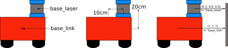
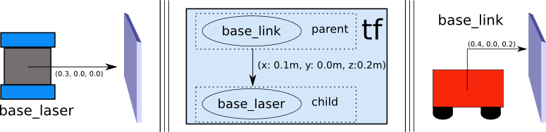
Volviendo al mundo real

Volviendo al mundo real

Denominación “de referencia” (padre) y “objetivo o target” (hijo)

Pose 2D

• Tres componentes: \((x, y, \theta)\)

\[ {}^W \boldsymbol{\xi}_R \sim {}^W\boldsymbol{T}_R = \begin{pmatrix} \cos{\theta} & -\sin{\theta} & {}^W t_x \\ \sin{\theta} & \cos{\theta} & {}^W t_y \\ 0 & 0 & 1 \end{pmatrix} \]

\[ {}^W\boldsymbol{\tilde{p}}_d = {}^W\boldsymbol{\xi}_R {}^R\boldsymbol{\tilde{p}}_d \]

• Se puede considerar como un movimiento de traslación y rotación del marco de coordenadas
• La pose de un marco de coordenada es siempre respecto a otro.

Pose 2D

Y si queremos ir del marco \(\{A\}\) al \(\{B\}\)?

La operación inversa

\[ {{}^A \boldsymbol{\xi}_B }^{-1} = {}^B \boldsymbol{\xi}_A \to {}^B \boldsymbol{T}_A = {{}^A \boldsymbol{T}_B }^{-1} \]

\[ \boldsymbol{\xi}^{-1} = \begin{pmatrix} \boldsymbol{R} & \boldsymbol{t} \\ \boldsymbol{0} & 1 \end{pmatrix}^{-1} = \begin{pmatrix} \boldsymbol{R}^T & -\boldsymbol{R}^T \boldsymbol{t} \\ \boldsymbol{0} & 1 \end{pmatrix} \]

Composición de poses

\[ {}^A\boldsymbol{\xi}_C = {}^A \boldsymbol{\xi}_B \otimes {}^B \boldsymbol{\xi}_C \]

Se puede cacular como: \[ {}^A \boldsymbol{\xi}_B \otimes {}^B \boldsymbol{\xi}_C = {}^A\boldsymbol{T}_B {}^B\boldsymbol{T}_C \]

\[ \boldsymbol{\xi}_1 \boldsymbol{\xi}_2 = \begin{pmatrix} \boldsymbol{R}_1 & \boldsymbol{t}_1 \\ \boldsymbol{0} & 1 \end{pmatrix} \begin{pmatrix} \boldsymbol{R}_2 & \boldsymbol{t}_2 \\ \boldsymbol{0} & 1 \end{pmatrix} \]

\[ \boldsymbol{\xi}_1 \boldsymbol{\xi}_2 = \begin{pmatrix} \boldsymbol{R}_1 \boldsymbol{R}_2 & \boldsymbol{t}_1 + \boldsymbol{R}_1 \boldsymbol{t}_2 \\ \boldsymbol{0} & 1 \end{pmatrix} \]

Convenciones (ROS Enhancement Proposals)

REP 103: “Standard Units of Measure and Coordinate Conventions”

• Unidades en S.I. (metro, segundo, kg, radian)
• Regla de la mano derecha
• Marcos ENU y NED
• Roll (X), Pitch (Y) y Yaw (Z)

REP = “Documentos que gobiernan ROS”

REP 103:

• Unidades: Sistema internacional -> Metros, kilogramo, segundo
• Radianes para ángulos
• Marcos de coordenadas: Todos son de mano derecha -> Cumplen la regla de la mano derecha
• La orientación de los ejes para cuerpos: x-adelante, y-izquierda, z-arriba
• Coordenadas geográficas de “corto alcance” -> ENU: X-este, Y-norte, Z-arriba
• Para sistemas de ambiente exteriores: -> NED:X-norte, Y-este, Z-abajo
• Rotaciones: Roll-Pitch-Yaw alrededor de X Y Z respectivamente

Convenciones (ROS Enhancement Proposals)

REP 105: “Coordinate Frames for Mobile Platforms”

• Convención de nombres
• Marco de coordenadas para plataformas robóticas
  • base_link: Fijo al robot (según REP103)
  • odom: Fijo al mundo (continuo, sin saltos, con drift)
  • map: Fijo al mundo (con saltos pero sin drift)

Nombramiento marcos de coordenadas: minúscula y con guión bajo para separación de palabras. Deben ser únicos

• ‘base_link’: Es el marco fijado rigidamente a la base del robot móvil -> Se recomienda utilizar lo del REP103
• ‘odom’: marco de referencia fijo respecto del mundo. Si bien sufre los problemas de drift sin límite, es continuo y no posee saltos.
• ‘map’: marco de referencia fijo respecto del mundo, con el eje Z apuntando hacia arriba. La pose del robot respecto del ‘map’ no debe tener un drift significativo a lo largo del tiempo. El marco puede no ser continuo, sufriendo saltos en cualquier momento.

Representación de rotaciones

Problemas con las matrices:

• 9 elementos (3D)
• Difícil de interpolar
• Acumulan errores (pueden perder ortogonalidad)
• Gimbal lock

Figure 1: Cuando el pitch (verde) y el yaw (magenta) se alinean, cambios en el roll (azul) y yaw aplican la misma rotación (Fuente: Wikipedia)

ROS 2 no usa matrices directamente para las rotaciones porque son grandes (9 números para una rotación), difíciles de interpolar, y pueden perder ortogonalidad al acumular errores.

Representación de rotaciones

Cuaterniones: Representación más compacta y robusta

\[ \boldsymbol{q} = \begin{pmatrix} x \\ y \\ z \\ w \end{pmatrix} \]

• Las poses ahora se componen de una traslación \(\boldsymbol t = \begin{pmatrix} x & y & z \end{pmatrix}\) y una orientación \(\boldsymbol{q}\)

En vez de eso, usamos cuaterniones, que representan la rotación de forma más compacta (4 números) y más robusta para cálculos computacionales. Así como en 2D usamos un solo ángulo (theta) para representar la orientación, en 3D usamos un cuaternión.

Representación de rotaciones

Ejemplo: \(\boldsymbol{p} = \begin{pmatrix} 1 & 0 \end{pmatrix}^T\) rotado \(90^{\circ}\)

Ángulo: \(\theta = 90^{\circ} = \tfrac{\pi}{2}\)

Matriz de rotación: \(\boldsymbol{R} = \begin{bmatrix} \cos{\theta} & -\sin{\theta} \\ \sin{\theta} & \cos{\theta} \end{bmatrix} = \begin{bmatrix} 0 & -1 \\ 1 & 0 \end{bmatrix}\)

Aplicamos: \[ \boldsymbol{p}' = \boldsymbol{R} \cdot \boldsymbol{p} = \begin{bmatrix} 0 & -1 \\ 1 & 0 \end{bmatrix} \begin{bmatrix} 1 \\ 0 \end{bmatrix} = \begin{bmatrix} 0 \\ 1 \end{bmatrix} \Rightarrow \boldsymbol{p}' = \begin{pmatrix} 0 \\ 1 \end{pmatrix} \]

Representación de rotaciones

Ejemplo: \(\boldsymbol{p} = \begin{pmatrix} 1 & 0 \end{pmatrix}^T\) rotado \(90^{\circ}\)

Cuaternion para rotación 2D: \(\boldsymbol{q} = \begin{pmatrix} x=0 & y=0 & z=\sin{ \tfrac{\theta}{2} } & w=\cos{ \tfrac{\theta}{2} } \end{pmatrix}\)

\[ \text{con} \, \theta = \tfrac{\pi}{2} \to z=\sin{ \tfrac{\pi}{4}} = \frac{\sqrt{2}}{2},\quad w=\cos{ \tfrac{\pi}{4} } = \frac{\sqrt{2}}{2} \]

Se escribe \(\boldsymbol{p}\) como cuaternion: \(\boldsymbol{p} = \begin{pmatrix} 1 & 0 & 0 & 0 \end{pmatrix}\)

Aplicamos:

\[ \boldsymbol{q} \circ \boldsymbol{p} \circ \boldsymbol{q}^{-1} = \begin{bmatrix} 0 \\ 0 \\ \frac{\sqrt{2}}{2} \\ \frac{\sqrt{2}}{2} \end{bmatrix} \begin{bmatrix} 1 \\ 0 \\ 0 \\ 0 \end{bmatrix} \begin{bmatrix} 0 \\ 0 \\ \frac{-\sqrt{2}}{2} \\ \frac{\sqrt{2}}{2} \end{bmatrix} = \begin{bmatrix} \frac{\sqrt{2}}{2} \\ \frac{\sqrt{2}}{2} \\ 0 \\ 0 \end{bmatrix} \begin{bmatrix} 0 \\ 0 \\ \frac{-\sqrt{2}}{2} \\ \frac{\sqrt{2}}{2} \end{bmatrix} = \begin{bmatrix} 0 \\ 1 \\ 0 \\ 0 \end{bmatrix} \Rightarrow \boldsymbol{p}' = \begin{pmatrix} 0 \\ 1 \end{pmatrix} \]

¿Por qué \(\theta / 2\)?

Porque los cuaterniones codifican media rotación internamente (por razones geométricas: la rotación se aplica como una conjugación, y termina duplicando el ángulo).

Librería de transformaciones

Por qué necesitamos una?

Ejemplo: un robot con dos marcos, uno el centro del robot ‘base_link’ y otro en el centro del laser ‘base_laser’. Dada la información respecto del laser ‘base_laser’, es necesario transformar esa información respecto al ‘base_link’ (definir una relación entre los dos marcos de coordenadas). Según la figura, será necesario aplicar una traslación (x: 0.1[m], y: 0.0[m], z: 0.2[m]), para ir del ‘base_link’ al ‘base_laser’. Como se requiere la transformación opuesta, sería (x: -0.1[m], y: 0.0[m], z: -0.2[m])

TF2 soluciona el problema de gestionar estas relaciones para que no lo tengamos que hacer por nuestra cuenta. Es útil sobre todo para escenarios no estáticos (99%).

Ejemplo extraido de docs.nav2.org

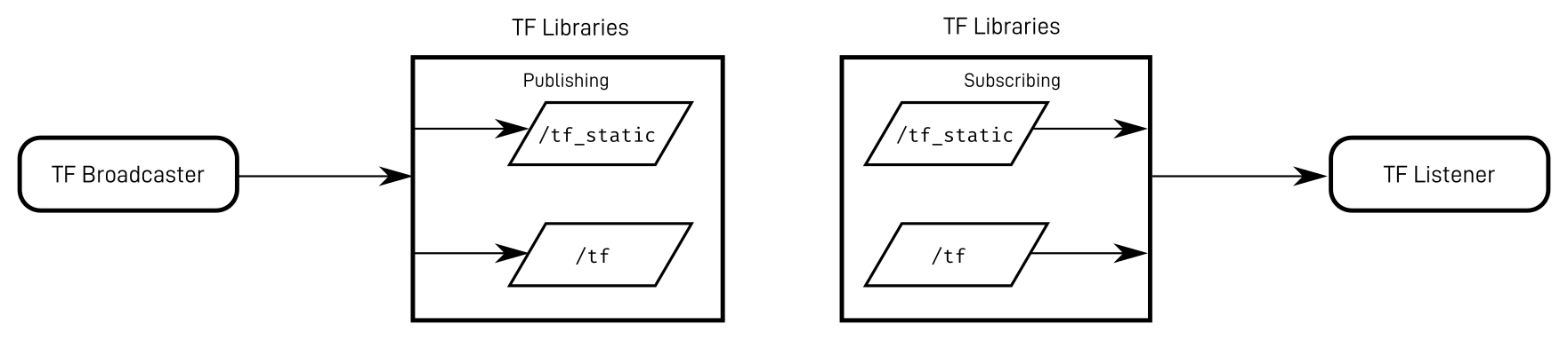
tf2: Librería de transformaciones

• Marco de coordenadas y sus transformaciones en el tiempo

• Estructura de árbol (no existen bucles)

• Herramienta para seguir los marcos de coordenada a través del tiempo (4ta dimensión)
• Mantiene las relaciones entre los marcos de coordenadas en una estructura de árbol buffereado en el tiempo
• Cada nodo en el árbol es un marco de coordenadas, y cada conexión o arista corresponde a la transformación que debe ser aplicada para ir o venir
• Arbol = no hay bucles = cada nodo 1 solo padre
• Cada marco puede estar definido solo por una transformación desde otro marco
• Permite transformar puntos, vectores, etc entre marcos de coordenadas para un determinado tiempo

tf2: Librería de transformaciones

• Basado en topics y mensajes tf2_msgs/msg/TFMessage

geometry_msgs/TransformStamped
├── std_msgs/Header header
├── string child_frame_id
└── geometry_msgs/Transform transform
    ├── geometry_msgs/Vector3 translation     ⬅️
    └── geometry_msgs/Quaternion rotation     ⬅️

• No se utilizan publishers/subscribers \(\to\) la librería tf2_ros

ROS representa orientaciones como cuaterniones en todos los mensajes de pose y transformaciones

Si bien se utilizan topics para manejar la comunicación, no se realiza una publicación/suscripción directa, sino a través de la librería por eso se dice broadcast/listen

tf2: Librería de transformaciones

• 2 Tipos de transformaciones: estáticas y dinámicas

Las transformaciones pueden ser estáticas o dinámicas (si cambian o no en el tiempo). En el caso de las transformaciones estáticas pueden publicarse una sola vez y se asumen “actualizadas” hasta que se transmita una nueva.

Fuente: articulatedrobotics.xyz

Transformaciones estáticas

Nodo static_transform_publisher

$ ros2 run tf2_ros static_transform_publisher

   x=[x] y=[y] z=[z]

   roll=[roll] pitch=[pitch] yaw=[yaw]

   [parent_frame] [child_frame]

Herramientas de visualización y análisis

• Ver el árbol: ros2 run rqt_tf_tree rqt_tf_tree

• Echo: ros2 run tf2_ros tf2_echo <marco_de_referencia> <marco_objetivo>

• Monitor: ros2 run tf2_ros tf2_monitor

• Visualización mediante RViz: ros2 run rviz2 rviz2

• Problemas comunes: que falte un transformación o que esté mal

Publicar transformaciones

Librerías

from tf2_ros import TransformBroadcaster
from geometry_msgs.msg import TransformStamped

# Conversión ángulos de euler a cuaternion (librería transforms3d)
from transforms3d.euler import euler2quat 

Completar las dependencias del paquete

<depend>tf2_ros_py</depend>

<depend>python3-transforms3d</depend>

Mediante el objeto TransformBroadcaster se podrán enviar las transformaciones

...
class FramePublisher(Node):
    def __init__(self):
        super().__init__('frame_publisher')

        # Inicializar el broadcaster
        self.tf_broadcaster = TransformBroadcaster(self)
...

Publicar transformaciones

Publicar transformaciones

...
    def send_tf(self):
        # Cálculo de los elementos de transformación
        # Transformación = Traslación + Rotación
        ...
        tf = TransformStamped()

        tf.header.stamp = self.get_clock().now().to_msg()
        # Marco de referencia (padre)
        tf.header.frame_id = 'world'  
        # Marco objetivo (hijo)                      
        tf.child_frame_id = 'robot'                 

        # Traslación
        tf.transform.translation.x = t_x
        tf.transform.translation.y = t_y
        tf.transform.translation.z = t_z

        # Rotación
        q = euler2quat(roll, pitch, yaw)  # Devuelve w x y z
        tf.transform.rotation.x = q[1]
        tf.transform.rotation.y = q[2]
        tf.transform.rotation.z = q[3]
        tf.transform.rotation.w = q[0]

        # Enviar la transformación
        self.tf_broadcaster.sendTransform(tf)

Laboratorio

Transformaciones 2D y tf2